Data analysis is a process of inspecting, cleaning, transforming, and modelling data with the goal of discovering useful information, informing conclusions, and supporting decision-making.

Data analysis can be break down into a few steps:

Create a hypothesis about some a given process (biological, economic, chemical, etc.)
Collect raw data to help us test the identified hypothesis.
Clean data. This often involves fixing or removing incorrect, corrupted, incorrectly formatted, duplicate, or incomplete data within a data set. (Obs. the degree of cleaning depends on several factors)
Perform preliminary analysis. This allow us to explore at trends, outliers, etc.
Analyze data and perform model diagnostics. By manipulating the data using various data analysis techniques and tools, you can begin to find trends, correlations, outliers, and variations that tell a story. Diagnostics help you determine if the assumptions of your model are reasonable.
Interpret the results of your analysis to see how well the data answered your original hypothesis.
Communicate your findings.

Image reference: www.r4ds.had.co.nz/introduction.html

What’s R?

R is a popular programming language used for statistical computing and graphical presentation. Its most common use is to analyze and visualize data.

What’s RStudio?

An integrated development environment for R, with a console, syntax-highlighting editor that supports direct code execution, and tools for plotting, history, debugging and workspace management.

What’s the difference between R and RStudio?

R and RStudio are not two different versions of the same thing. One can’t be substituted for the other.

But they work together. R is a programming language for statistical calculation. RStudio is an Integrated Development Environment (IDE) that helps you develop programs in R.

In this workshop, we will be working mostly with RStudio.

Why not Excel?

Here is a reason why….

Source: https://www.educba.com/errors-in-excel/

Why use R (or RStudio)?

It is a great resource for data analysis, data visualization, data science and machine learning
It provides many statistical techniques (such as statistical tests, classification, clustering and data reduction)
It is easy to draw graphs in R, like pie charts, histograms, box plot, scatter plot, etc++
It works on different platforms (Windows, Mac, Linux)
It is open-source and free
It has a large community support
It has many packages (libraries of functions) that can be used to solve different problems

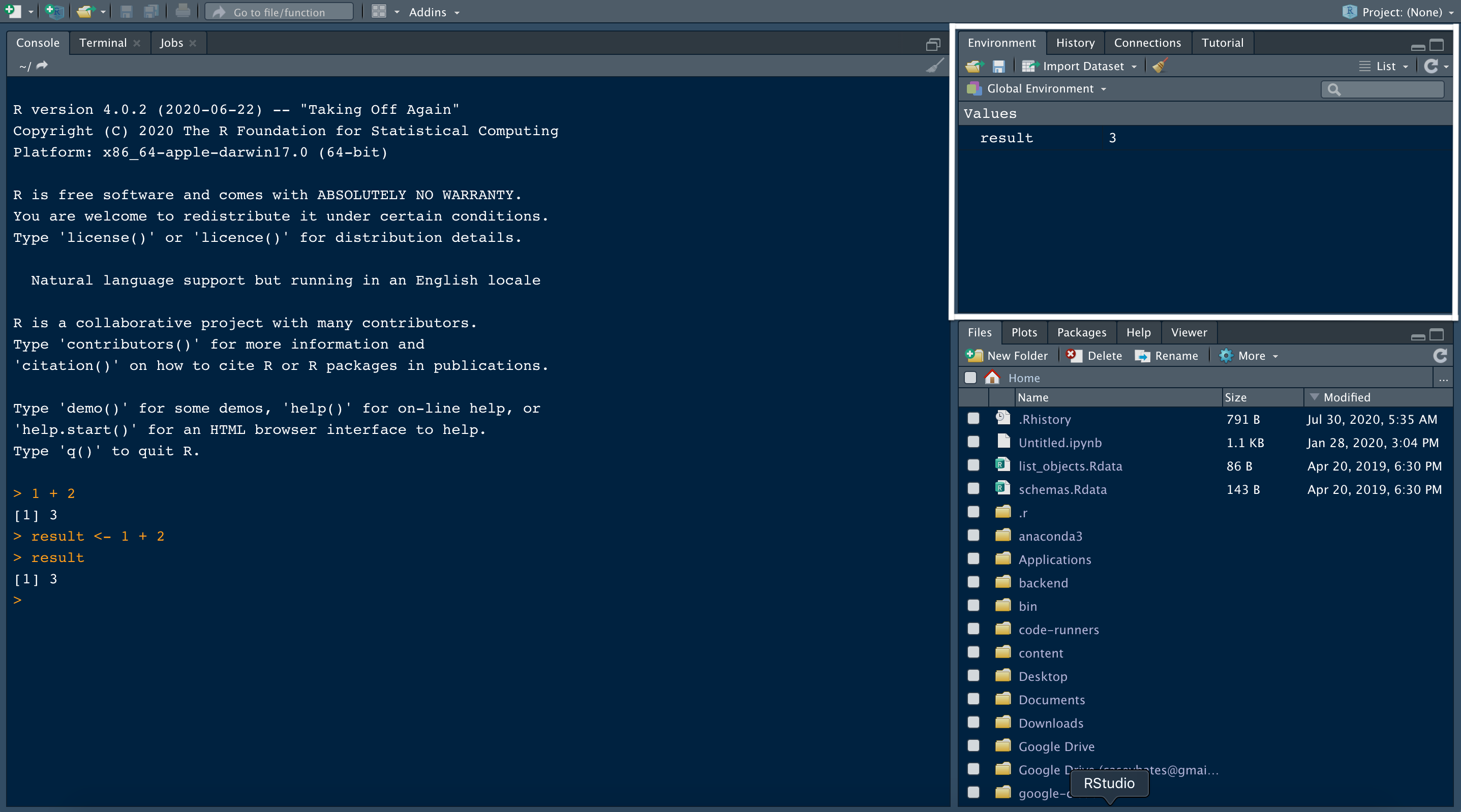
RStudio

When we open RStudio for the first time, we’ll probably see a layout like this:

RStudio view. Image reference: www.dataquest.io/blog/tutorial-getting-started-with-r-and-rstudio/

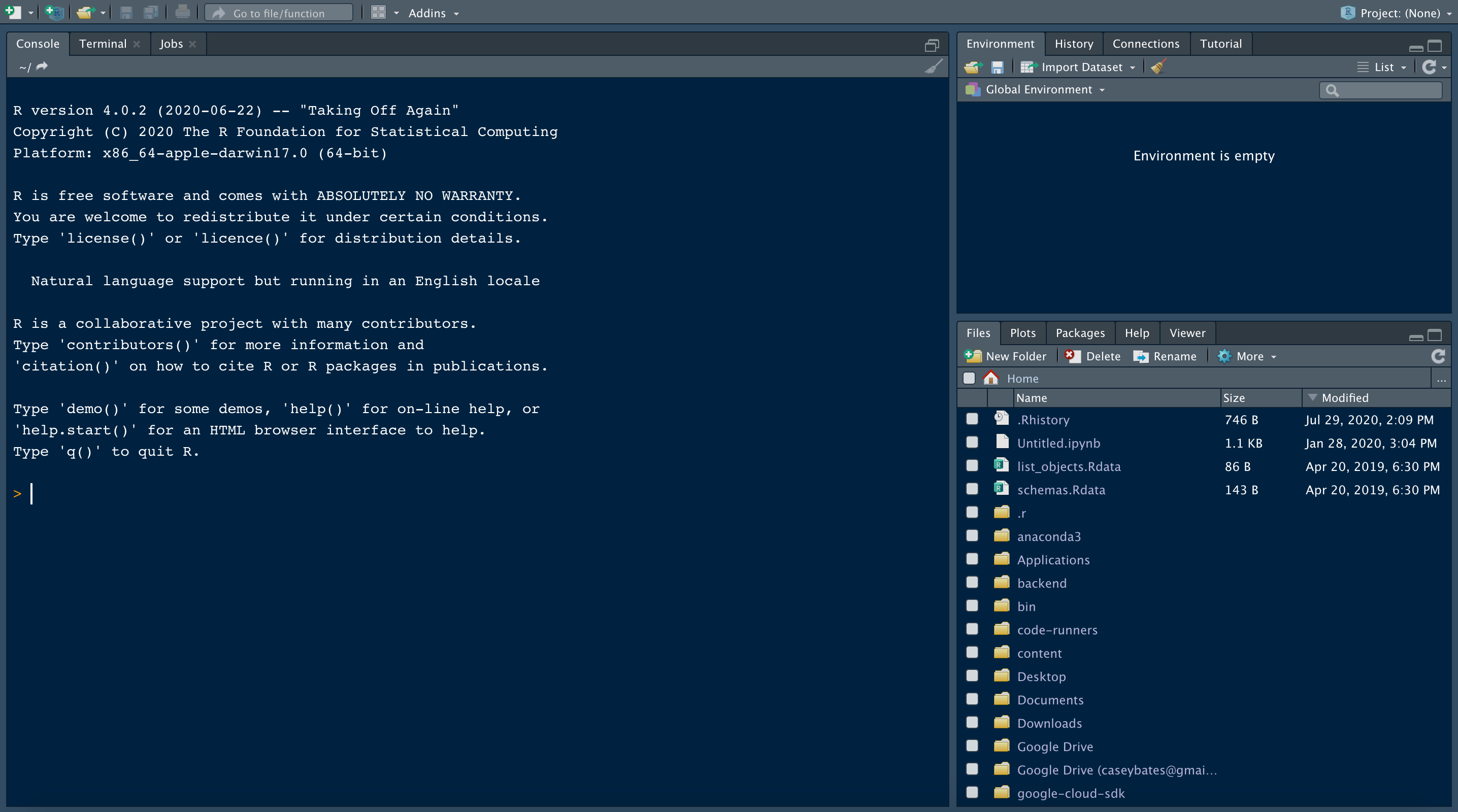
Console

Let’s start off by introducing some features of the Console. The Console is a tab in RStudio where we can run R code.

Notice that the window pane where the console is located contains three tabs: Console, Terminal and Jobs (this may vary depending on the version of RStudio in use). We’ll focus on the Console for now.

When we open RStudio, the console contains information about the version of R we’re working with. Scroll down, and try typing a few expressions like this one. Press the enter key to see the result.

Console. Image reference: www.dataquest.io/blog/tutorial-getting-started-with-r-and-rstudio/

Please, go ahead and type this into your Console:

1 + 2

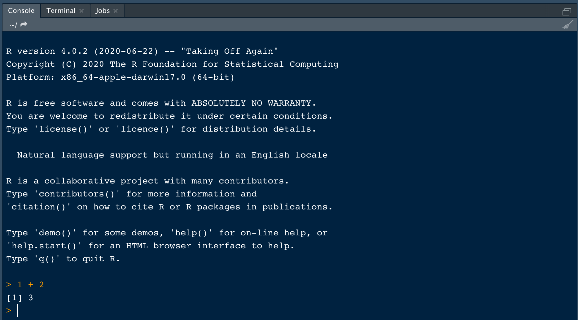
result <- 1 + 2

result

We’ll see any objects we created, such as result, under values in the Environment tab. Notice that the value, 3, stored in the variable is displayed.

Sometimes, having too many named objects in the global environment creates confusion. Maybe we’d like to remove all or some of the objects. To remove all objects, click the broom icon at the top of the window:

The Global Environment

We can think of the global environment as our workspace. During a programming session in R, any variables we define, or data we import and save in a dataframe, are stored in our global environment. In RStudio, we can see the objects in our global environment in the Environment tab at the top right of the interface:

Global environment. Image reference: www.dataquest.io/blog/tutorial-getting-started-with-r-and-rstudio/

We’ll see any objects we created, such as result, under values in the Environment tab. Notice that the value, 3, stored in the variable is displayed.

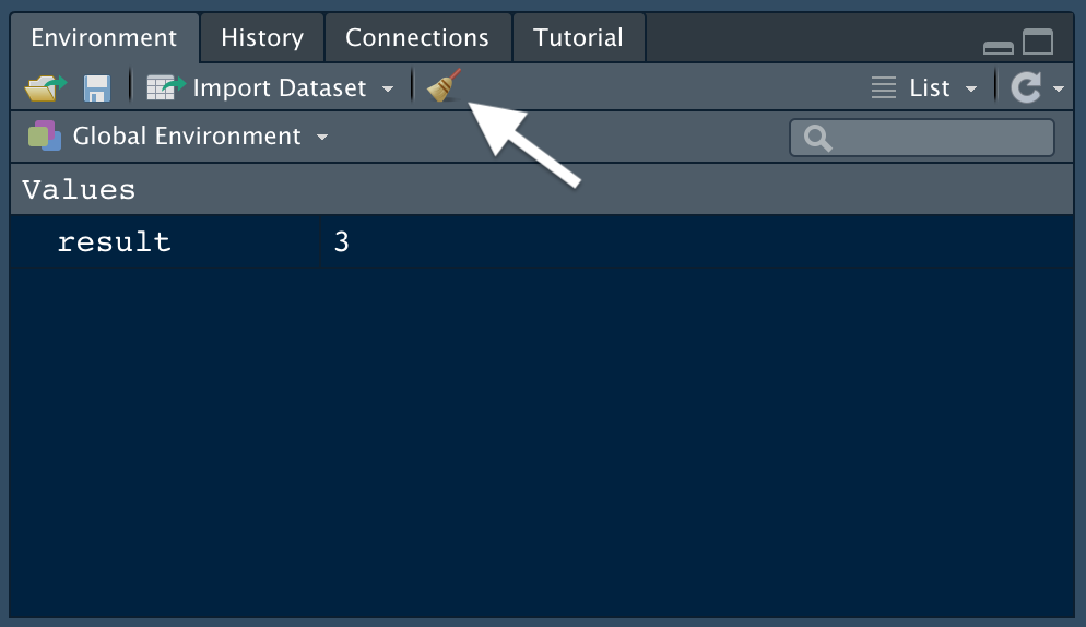
Image reference: www.dataquest.io/blog/tutorial-getting-started-with-r-and-rstudio/

Hands-on with R

In this section we will investigate the following questions: [[ How does R understand data? ]]

How to use this script and R
Creating objects and using logicals
Sequences and vectors (1-D)
Data frames, basic data manipulation (subsetting, renaming, joining), and finding help for using functions

Step 1: How to use this R script

Copy and paste the following into the console and run it:

print("the instructors' names are Vinny and Danielle")

Run a single line of your script in the console by placing your cursor on the line you want to submit and use your cursor to press the “Run” button at the top right. You can also use the shortcut key strokes cmd+enter (mac) or ctrl+enter (PC) to run a single line at a time.

The two other most important keyboard shortcuts that you’ll want to use are the Tab key to auto-complete your typing at the command line and ctrl+up arrow or cmd+up arrow to access the most recently typed commands.

You can also select only part of a line to have it run on the console.

Let’s do an exercise:

Exercise 1: Use the function print to print the sentence.

a = c("my name is ____")

print(a)

It’s important to realize that when you run code as we’ve done above, the result of the code (or value) is only displayed in the console

You always can see what the function is via this:

?print

R can also be used to perform calculations, such as the following:

2+2
4*20
5+1/3

Does the last one seem right?

What rules does R apply for the order of operations and how do you find out?

Let’s modify the statement above to see if adding parentheses changes the result:

(5+1)/3

Does it matter if there are spaces added into this?

 ( 5 + 1 ) / 3

That shows us that the spaces did not matter for the calculation.

R also has some pre-defined mathematical terms that you can use, such as pi.

What is pi times pi ?

pi*pi

pi^2 #this does the same thing because ^ is, here, interpreted as "taken to the exponent"

Other mathematical functions include:

log(1) 
sqrt(4)
exp(1) 
exp(1)

Step 2: Creating objects and using logicals

At the heart of almost everything you will do (or ever likely to do) in R is the concept that everything in R is an object. Objects are like shortcuts. Having the ability to manipulate objects in R makes things very handy. Objects are stored in the environment tab (check it out). They are a way to store data without having to re-type them. By virtue, objects are only created once something has been assigned to them. Anything can be stored in an object, including figures, lists!

Let’s repeat our simple math calculation above, this time using objects. If we want to calculate (5+1)/3 using objects, it needs to look like this: (a+b)/c The objects a, b, and c do not exist yet, so we need to assign values to them in order to create them. R interprets the less than symbol and dash as “assign”. So we need to do the following:

a <- 5 #assign the number 5 to an object called a
b <- 1 #assign number 1 to object b
c = 3 # we can also use `=` to assign 3 to c. But `<-` is the preferred assignment operator as `=` is used to call arguments in function calls.

As you are assigning these numbers to objects, they appear in your environment (top right). These objects are not being saved to a hard drive, they are stored in memory of your computer only.

NOTE if you assign something to an object that already exists, R will do what you tell it and overwrite that object with the new assignment.

Now we can execute our calculation using objects instead of numbers. Try it!

(a+b)/c

Avoid creating object names that start with a number because R will look at the first character and try to interpret the entire name as a mathematical term. Try this:

2foxes <- 1

The error here tells us that something went wrong and R cannot proceed.

If we want to assign (a+b)/c to a new object called answer – what will the object contain? Find out:

answer <- (a+b)/c

Take a look at the object answer by typing the name into the command line:

answer

What would you get if you multiplied answer by 2?

answer*2

Let’s now look into other examples about the use of vectors. This is going to be important in later data manipulation steps. John, a made-up character, recently weighted himself and found the value below.

john_weight_kg <- 86.18

Wait. John lives in the US where imperial units are used instead of international units. Let’s change that to lb (1kg is equivalent to approximately 2.2 lb). How can we transform John’s weight in lb?

john_weight_lb = 2.2 * john_weight_kg #(weight in pounds is 2.2 times the weight in kg)
john_weight_lb

Now,let’s calculate John’s body mass index. Body mass index (BMI) is a measure of body fat based on height and weight that applies to adult men and women. John is 5’9 feet tall. That equates to 69 in. The formula for BMI calculations is weight (lb) / [height (in)]2 x 703.

BMI = john_weight_lb/(69^2)*703
BMI

We can also use logical operations in R. The answer to a logical question is always TRUE or FALSE.

Is a greater than b?

a > b #You can look at the Values on your right to check the answer.

Is b greater than 10?

b > 10

Is b + c greater than a?

b + c > a

R will first evaluate the algebraic operation (+) and then evaluate the logical operation (>). So, we don’t need to use (b+c) > a.

Is a equal to 7?

a = 7

Oops! We did not get any answer. What went wrong? Let’s print a.

a = 7 changed the value of a to ‘7’. So, how do we find if a is equal to ‘7’?

a == 7 #We need to put two '=' signs to check equality.

Is a not equal to ‘7’?

a != 7

Are both a and b greater than c?

(a > c) & (b > c)

Is either a or b greater than c?

(a > c) | (b > c)

The examples above dealt with numeric values assigned to objects. We can also store character data in objects. We need to place the character data (words, phrases, etc.) inside quotation marks, otherwise R will try to interpret the character data as an object and will produce an error.

Let’s use my name for this exercise. Let’s create two objects, one for my first name and another for my last name.

first.name <- "Vinny"
last.name <- 'Garnica' #Single quotes work too!

Notice that we have enclosed the string in quotes. If you forget to use the quotes you will receive an error message

first.name <- Vinny

We now have those two objects. Let’s look at them.

first.name
last.name

Since we each have a first name and a family name, let’s do another exercise.

Exercise 2: Modify the objects first.name and last.name so that instead of my name, they contain your name.

first.name <- "____" #Replace ____ with your own name
last.name <- "____"

Did this work? Let’s look at the two objects:

first.name
Last.name

Oops! What went wrong? R is case-sensitive, so last.name is interpreted differently than Last.name. Let’s try again:

first.name
last.name #It works!

Using a function c() we can tell R to combine these two objects. This function will combine values from the first object with the second object and return them as a single observation. Let’s try it:

c(first.name, last.name)

What about:

first.name+last.name

The error message is essentially telling you that either one or both of the objects first.name and last.name are not a number and therefore cannot be added together.

Notice how the names are returned inside quotation marks, which tells us that these are interpreted as character data in R. You’ll also notice that each name is placed inside quotes and that’s because c() combined names into a single vector that contains two elements, your first and your last name. This brings us to the next step in our introduction, vectors.

Step 3: Vectors, functions, and sequences

Up to here, the objects we’ve created only contained a single element. You can store more than one element in a 1-dimensional object of unlimited length. Let’s create an object that is a vector of our first and last names using the two objects that we created previously.

Avoid re-typing your commands. Since the last command that we ran contained what we want, we can simply use the up arrow to access the most recently submitted command and modify it. You can also access the History tab in the top right panel of RStudio or, at the command line, access a list of the most recent commands using the cmd + up arrow OR the ctrl + up arrow.

name <- c(first.name, last.name)

We can inspect this object by typing name at the command line. We can inspect the structure of this object using the function str() on name.

str(name)

This shows us that this is a vector because the elements in it are ordered from 1 to 2 as shown by the [1:2]. This also tells us that this list is a character list, which is indicated by the chr label. We also see the two elements in this vector, which is your first and last name.

What is the length of your name? We can find out using the function length()

length(name)

Let’s work with another vector. In the code below, you are going to created an object called my_vec and assigned it a value using the function c().

my_vec <- c(1,5) #ask students to come up with 5 numbers

Again, at this time, you know how to get my_vec.

my_vec

Let’s obtain the mean of my_vec? How? Using mean() function. We also want to get a measurement of dispersion, the variance through var() and the standard deviation via sd().

mean(my_vec)
var(my_vec)     
sd(my_vec)

We know that our vector my_vec contains 5 elements. We can access that via the length function.

length(my_vec)

Let’s quickly see the same example with missing data. In R, missing data is usually represented by an NA symbol meaning ‘Not Available’. Data may be missing for a whole bunch of reasons, maybe your machine broke down, maybe you broke down, maybe the weather was too bad to collect data on a particular day etc etc. Missing data can be a pain in the proverbial both from an R perspective and also a statistical perspective.

For example, let’s say we collected air temperature readings over 10 days, but our thermometer broke on day 2 and again on day 9 so we have no data for those days

temp  <- c(7.2, NA, 7.1, 6.9, 6.5, 5.8, 5.8, 5.5, NA, 5.5)
temp

We now want to calculate the mean temperature over these days using the mean() function

mean_temp <- mean(temp)
mean_temp

Flippin heck, what’s happened here? Why does the mean() function return an NA? Actually, R is doing something very sensible (at least in our opinion!). If a vector has a missing value then the only possible value to return when calculating a mean is NA. R doesn’t know that you perhaps want to ignore the NA values (R can’t read your mind - yet!). Happily, if we look at the help file (use help("mean") - see the next section for more details) associated with the mean() function we can see there is an argument na.rm = which is set to FALSE by default.

mean_temp <- mean(temp, na.rm = TRUE)
mean_temp

Changing gears…. Sometimes it can be useful to create a vector that contains a regular sequence of values in steps of one. Here we can make use of a shortcut using the : symbol.

my_seq <- 1:10
my_seq

my_seq2 <- 10:1
my_seq2

Other useful functions for generating vectors of sequences include the seq() and rep() functions. For example, to generate a sequence from 0 to 20 in steps of 2

my_seq2 <- seq(from = 0, to = 20, by = 2)
my_seq2

The rep() function allows you to replicate (repeat) values a specified number of times. To repeat the value 2, 10 times

my_seq3 <- rep(2, times = 10)
my_seq3

Now, let’s work through another handy example. Let’s create three objects to represent today’s date in numbers for the month (10), day (28), and year (2022).

month <- 10
day <- 28
year <- 2022

Combine those three objects using the c() function:

today <- c(month, day, year)

Inspect this object by typing the name today at the command line. Let’s take a look at the structure of today. Obs. why knowing str is so important?

str(today)

You’ll notice that the vector has three elements [1:3] and it contains only numeric data.

Let’s do the same thing using the name October for month and see how that changes our vector. Notice that we are not modifying the object month, we are simply combining our two existing objects with the word “October”.

c("October", day, year)

In this case we didn’t re-assign the object named today. To inspect the structure of this vector, we can wrap the statement within the str() function, as shown below. We also want to inspect the data class (ie. whether numeric or character) using the function class(). Don’t forget to use the up-arrow to access the last like that you ran!

str(c("October", day, year)) #this shows us the structure of the object
class(c("October", day, year))

Notice how R is trying to keep our data organized according to type. Rather than coding this vector as containing numbers and characters, it has decided that because it can’t call everything in our vector a number that it will call everything characters. This process is called coercion.

Let’s say we wanted to create a table that showed every date this month:

We know there are 31 days in the month, so we can modify the object day to contain all of the 31 days in this month. You see at in the console that this created a sequence of 31 numbers from 1 to 31. Let’s go ahead and assign this to the object day.

day <- 1:31

For the objects month and year, we don’t need to modify them, however, we want to repeat each of them a total of 31 times because we need to repeat each, once for each day.

We can easily repeat the number 10 a total of 31 times using the function rep(), specifying how many times we should repeat this object. Let’s assign 10 to month and modify the object month to contain 31 copies.

month <- 10
month <- rep(month, times = 31)
month

Let’s check to make sure that month is correct using the function length():

length(month)

There are 31 elements in this vector and we can inspect individual elements in the vector based on their ordered position using square brackets:

month[28] #the number inside the brackets corresponds to location of element in list, not value
day[28]

In this case, the 28th element in month is 10, and the 28th element in day is 28 which confirms that we created this correctly.

Type day[32] into your R console. What do you get? What does it mean? Ask yourself the question, “Are there any months with 32 days?”

We can create the object year to contain 31 repeats of 2022, however, this time, let’s say we wanted to make sure that this object was always the same length as the number of days we have in a month. Instead of specifying 31, we can simply get that information using the length() function. Here, we’ll replace 31 with length(day), which is equivalent.

year <- rep(2022, times = length(day))
year
length(year)

We now have three vectors to create our table and they are exactly the same length:

length(day)
length(month)
length(year)

Step 4: Data frames, basic data manipulation, and finding help

Remember that our goal here is to create a table with the columns “month”, “day”, and “year”. First, here’s a quick reminder of what we want this to look like:

   day   month   year
   1     10       2022
   2     10       2022
   3     10       2022
   ...

In order to create a data frame, we can use the command data.frame(). This function will create columns out of vectors that are all the same length. In the function, we just have to specify name of the column and populate it with vector data.

October <- data.frame(day = day, month = month, year = year)

Let’s inspect this new object in the same way as vectors:

October
length(October)

Using the length() function, we see it says 3. This is because October has three columns: day, month, and year. A data frame is a two-dimensional object which stores its information in rows and columns.

Because this is a 2-dimensional object, we can inspect the dimensions using the dim() function:

dim(October)

This tells us that we have 31 rows and 3 columns. R also provides the nrow() and ncol() functions to make it easier to remember which is which:

nrow(October)
ncol(October)

What happens when we use the str() function?

str(October)

We can see that it’s listing the columns we have in our table and showing us how they are represented. Notice the $ to the left of each column name, this is how we access the columns of the data frame:

October$day
October$month
October$year

You can see that these are the same as the vectors we created earlier.

Because this object is rather large, we didn’t get to see the top rows of the object. A quick way to look at the top of the object is with the head() function and if we wanted to look at the bottom, we would use tail().

head(october) #if this didn't work, double-check that you spelled the object name correctly

Now that we have our table, the question becomes, how do we inspect different elements?

Just like we can inspect the 28th element in the day vector using day[28], we can also use the brackets to subset a table, the only catch is that we have to use the coordinates of the row(s) and the column(s) we want. We can do this by specifying [row, column]. These are analagous to X and Y Cartesian coordinates. Let’s take a look at the elements in the 28th row, separately:

October[28, 1] #day
October[28, "month"] #you can use characters when the elements are named!
October[28, 3] #year
October[28, -3] #here `-` means all columns except the third (year)
October[28, -2] #day and year

If we don’t specify a dimension, R will give us the entire contents of that dimension. Let’s look at the row that contains today’s date:

October[28, ]

You can also use this to access just one column of the matrix. Let’s look at month:

October[, 2]

Now that we’ve inspected the object October, let’s create the same thing for the month of November. How should we do this?

One option would be to create new objects for day, month, and year and combine them just like we did for October. What is the simplest method to do this, using the fewest number of steps?

We can simply make a copy of October and add two vectors with information about the 30th and 31st days. Let’s do this step by step. Note that November contains 30 days. We can re-do all the operations above, making sure that we remove the 31st day of the process or copy October and remove the 31st day.

November <- October
November <- November[-31,]

Inspect what we have now:

str(November) #we have an extra column
tail(November) #we only have 31 days

We need to change the month column so that it says 11 instead of 10, how can we do this? Let’s just look at the column first:

November$month

We need to add 1 to each of these values, so let’s try that!

November$month + 1

This worked, so now we just need to replace values in November[,2] with the new expression:

November$month <- November$month + 1  #Did it work?
str(November)

Let’s combine both of these tables into an object called ‘Fall’. You know what function to use, right?

Fall <- rbind(October, November)

Inspect this object to ensure it was made correctly.

str(Fall)
head(Fall)
tail(Fall)

We now have a new object Fall that contains only numeric data. Let’s revise this object so that it uses names for the month instead of numbers. We want it to look like this:

   day   month    year
   1     October  2022
   2     October  2022
   3     October  2022
   ...

Months need to be changed from the number 10 to “October” and from 11 to “November” in the second column. Let’s first look at the month column.

Fall$month

We want to specify only the cells in this list that are 10. We know that rows 1 to 31 contain 10’s and the rest contain 11’s, which means we can inspect those rows in the object Fall:

Fall[1:31, "month"]  #October
Fall[-c(1:31), "month"] #November

Notice that we used -c(1:31), what do you think this is doing? Why would this give us the values for the month of November?

We can use the ifelse() function to replace the values in our column. How do we use this function? A good first step to figuring out how you can use a function is to look at its help page. The way you can do that is by typing either help("function_name") or ?function_name.

?ifelse

Exercise 4: Type ?ifelse and answer these three questions: 1. What does it do? (Description) 2. What are the arguments? (Usage/Arguments) 3. What does it return? (Value)

In order to use ifelse, we will need to provide three things:

A logical question about the elements of an object : Fall$month == 10
Values for TRUE elements : “October”
Values for FALSE elements : “November”

ifelse(Fall$month == 10, yes = "October", no = "November")

Fall$month <- ifelse(Fall$month == 10, yes = "October", no = "November")

Notice that we had to use == to indicate equality. This is so that R doesn’t get confused and assume we are using the argument assignment, =.

Now, let’s inspect Fall.

str(Fall)
head(Fall)
tail(Fall)

Let’s change first letter of every column name to uppercase i.e., replace “day” with “Day” and so on. We can do this using colnames() function.

colnames(Fall) #Current column names
colnames(Fall) <- c("Day", "Month", "Year") #New column names

Let’s inspect Fall again.

str(Fall)
head(Fall)

Recap

R has many functionalities that make data management more enjoyable.
Mathematical operations: +, -, /, >, |, and the use of ()
Difference between = and ==.
Mathematical functions: log(),sqrt(),exp(), and others…
Functions: print(), str(), length(), mean(), var(), sd(), rep(), class(), data.frame(), head(), tail(), dim(), nrow(), ncol(), ifelse(), colnames().

References

APS_IntroR_Workshop - Dr. Sydney E. Everhart, Nikita Gambhir, Dr. Kaitlin Gold, Dr. Lucky Mehra, Dr. Zhian N. Kamvar, and Dr. O. William McClung.

An Introduction to R - Alex Douglas, Deon Roos, Francesca Mancini, Ana Couto & David Lusseau.

Part1 - Introduction